LIBS Info: Tutorial 3: Exploring AtomAnalyzer for LIBS analysis
Disclaimer
I have no association with Atom Trace and obtained no benefit from writing this Tutorial. As the only free LIBS software I could find, the product warrants some investigation to see what it offers.
Getting the Software
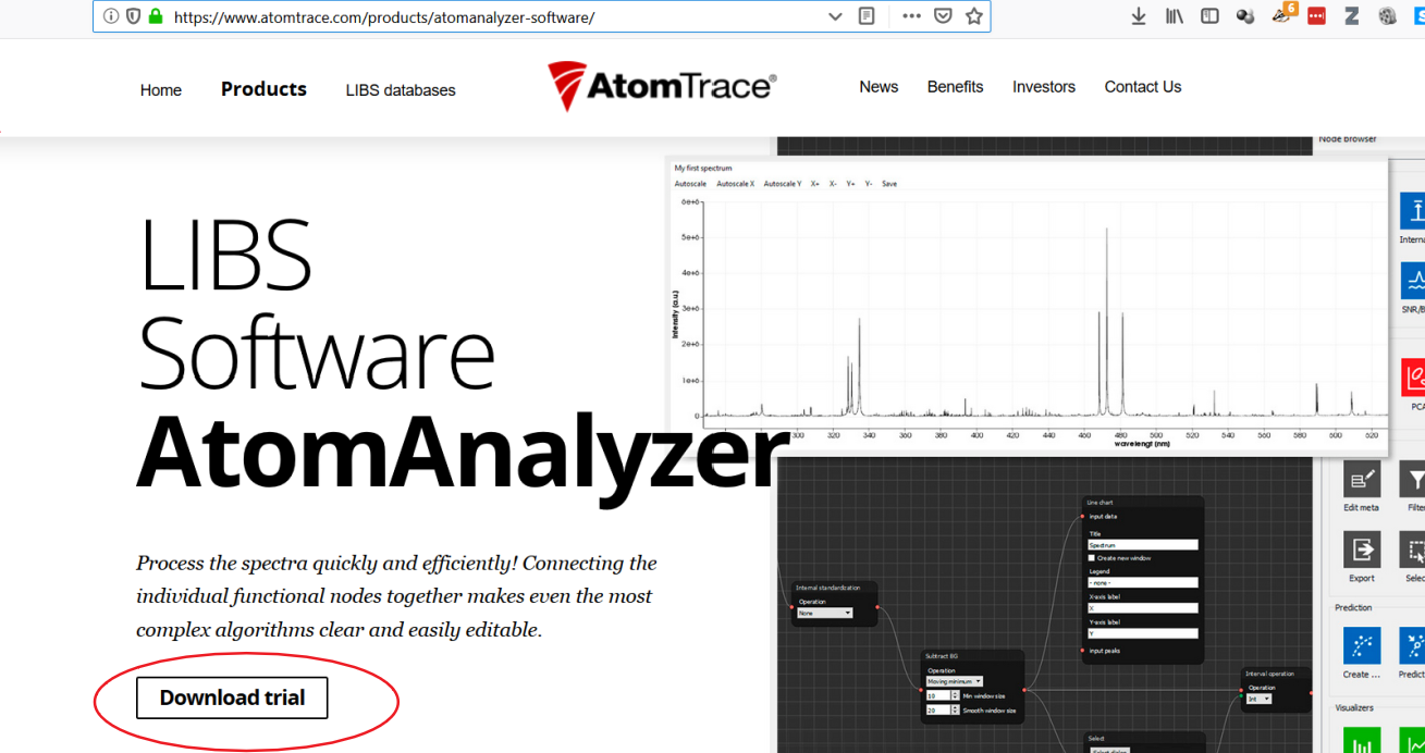
Navigate to the Atom Trace Software Site
To get the software you need to register, but to date I haven't received any spam from them!
Put in an email address and a password. As this becomes your ID for the software, remember these
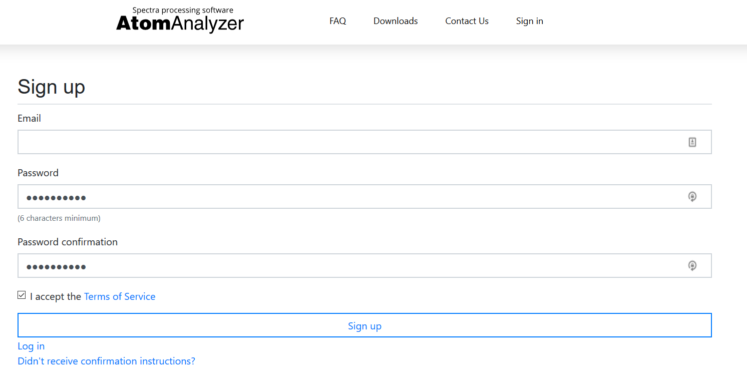
An email will be sent to the email address provided with registration instructions (clicking on a link in the email or copying a URL to your browser)
Once you have logged in using the email address/password entered at registration, click the Get Free Trial button
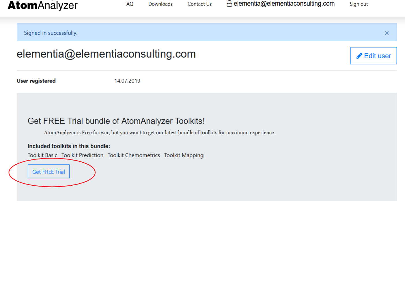
Once clicked the you will be issued with download buttons for the AtomAnalyzer Software and the necessary toolkits to do the analyses. The Toolkits have one month licenses
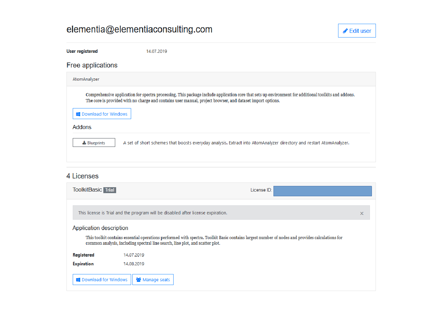
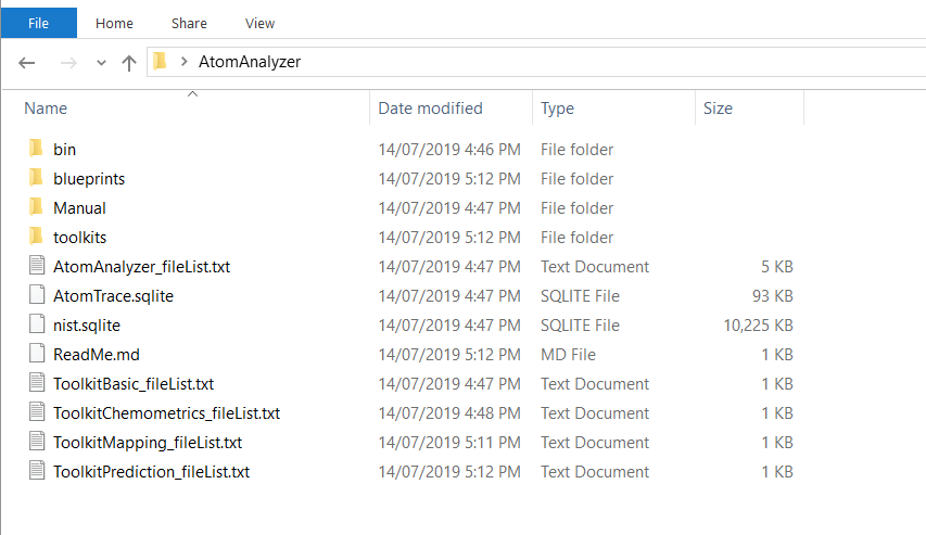
We will only be using the Toolkit Basic, but it is worth downloading them all at this time (as well as the blue prints). The toolkits are less than 1Meg. The AtomAnalyzer Software is 72.5M. All the downloads are zip files. Make a directory and extract them all into that directory. At the end, it should look something like this
Running the Software
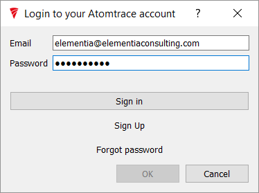
The AtomAnalyzer software is in the /bin directory. Run the software.
The first time it runs, enter the email address and password that was used during signup
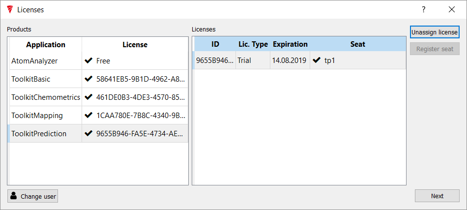
Once signed in, for the software to work the licenses that were issued need to be applied to this version of the product.
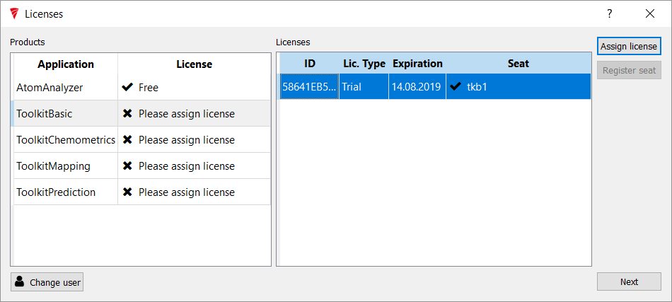
Work down the list, assigning licenses until all the lines are filled
Making a calibration curve
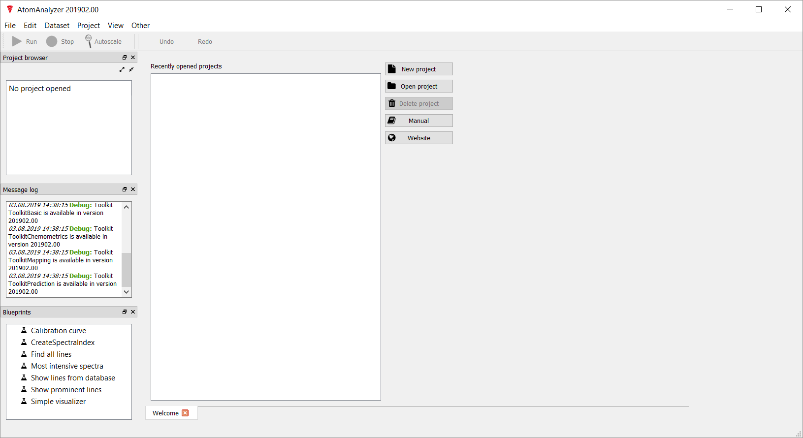
On opening the software, the screen looks like this
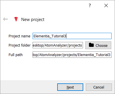
All analysis work happens in a project, so make a New Project by clicking the button. Give the Project a meaningful name, andclick Next
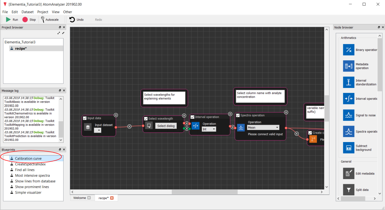
Double click on recipe in the list on left of the screen. This will change the screen to include the grid on which we will construct the calibration curve. AtomAnalyzer is similar to NodeRed or Lab View in that a complicated analysis flow is constructed by wiring together nodes which perform the key tasks.
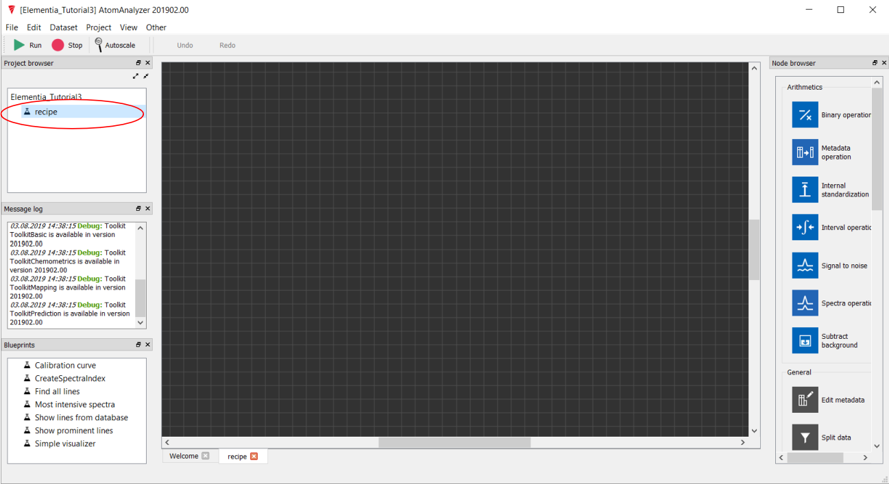
For this tutorial we will construct a calibration curve.
From the Blueprints section drag a Calibration Curve onto the black grid (work surface). This will select and wire the correct nodes for this analysis
Adding the Spectra
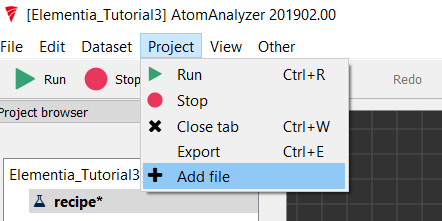
Now that we have a method, we need some spectra to analyse. From the Project Menu choose Add File
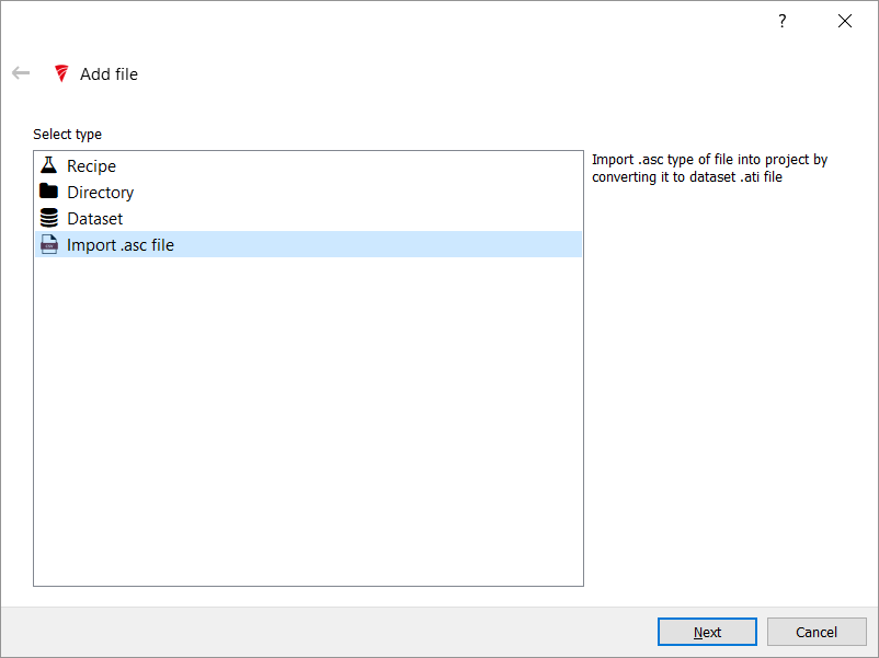
In this case, we are going to add a .csv file which contains the spectra data. To import this, choose the Import .asc file option and click Next
Click the Add File button and select the source file. If you are doing this tutorial from the Elementia Consulting Github then the file we are using for this work is in the files directory (OREAS_source_h.csv).

Click Next
Adjust the settings to match the following image - that is, change the Column, Skip Columns, Maximum Dimensions: Rows & Columns. Press Commit
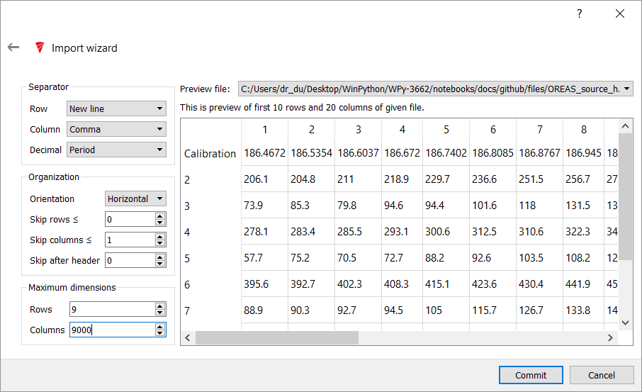
If all the settings are correct, the data will import and you can clic Finish on the next screen.
This has added the spectra to the Project, but we need to associate the element concentrations (in this case Na) with the spectra. Double click the data file in the Project Browser.
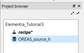
Change to the Data Metadata tab
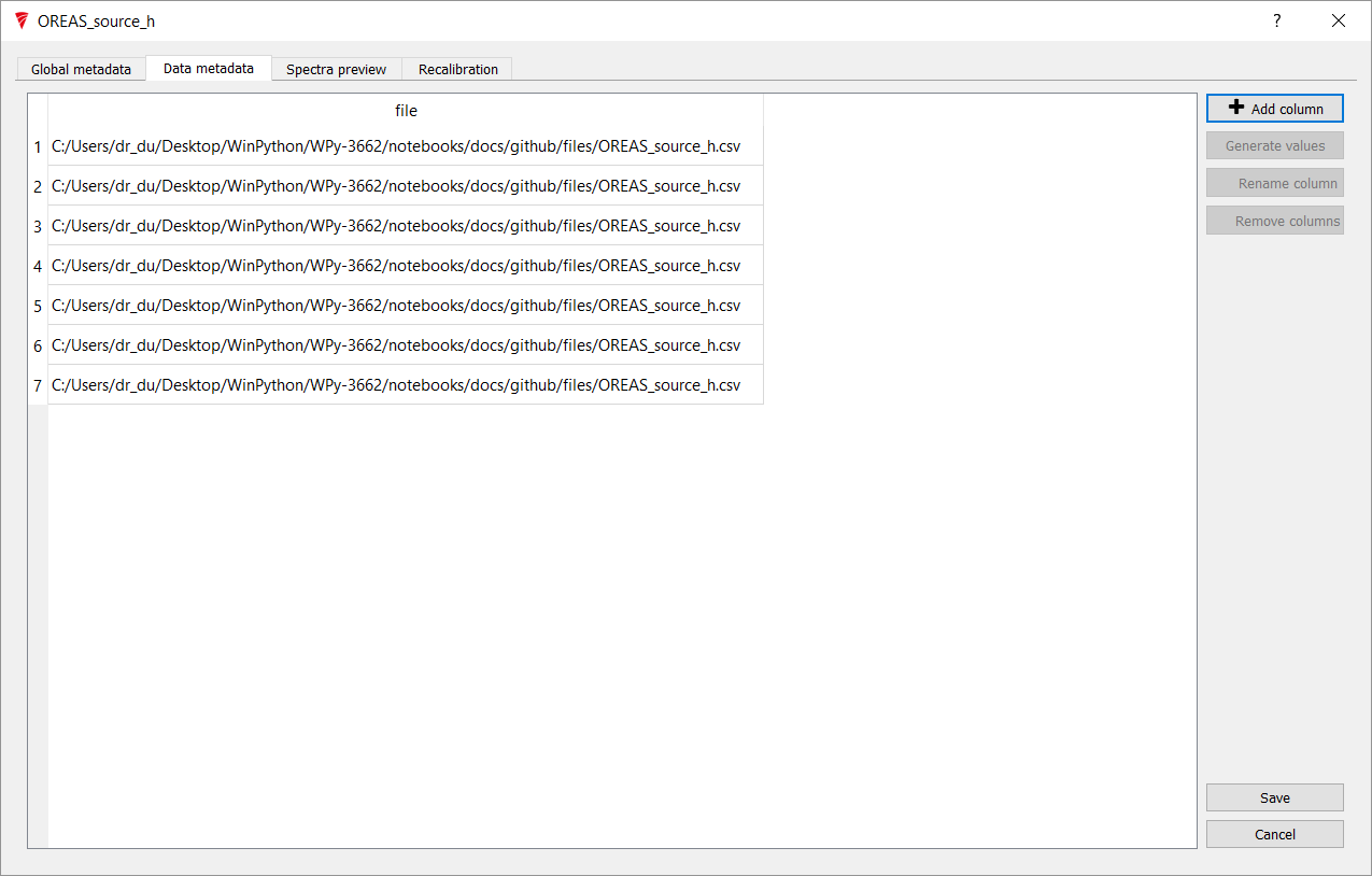
Click Add Column
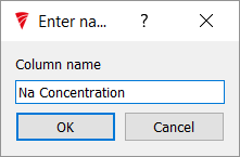
Choose it a name that will be meaningful for future use. Here I have chosen 'Na Concentration'.
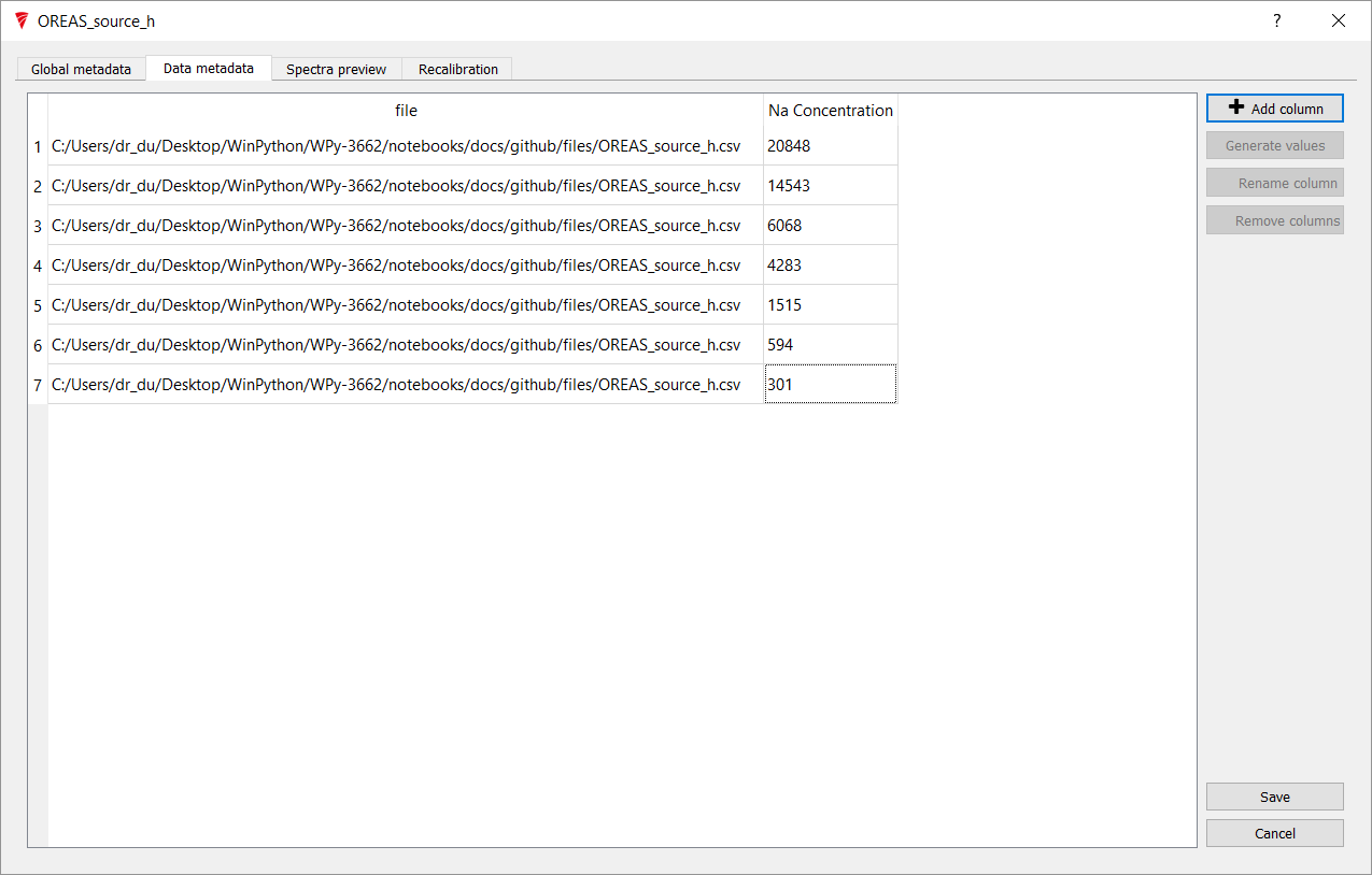
Fill in the concentration values and then press Save.
Building the Calibration Curve
Return to our recipe nodes, we can starting setting these up.
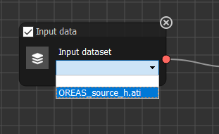
On the first node (Input Data), our source data should now be available from the drop down menu
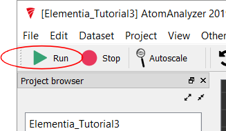
Now press Run - this will mean that the first node sends its data to the next one.
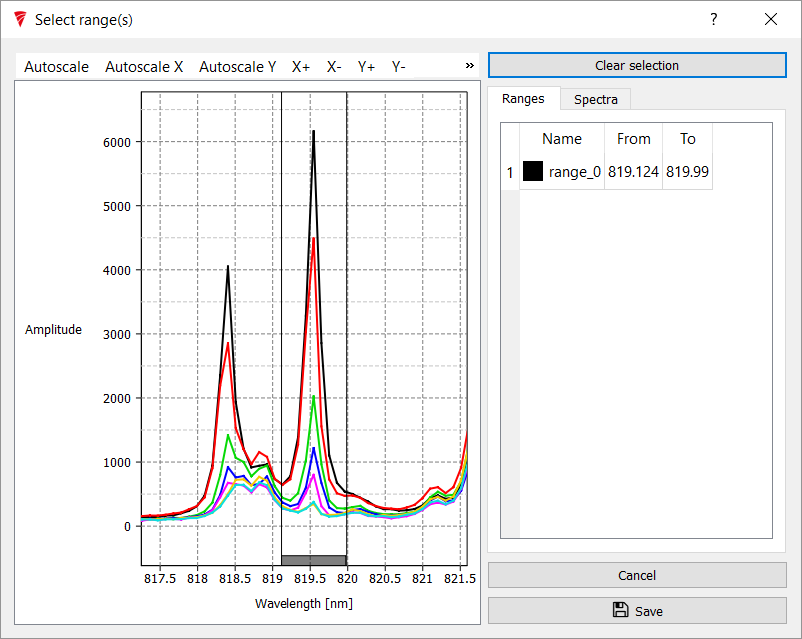
For this analysis we will use the Na peak at 819.4nm that we worked with last Tutorial. On the Select Wavelength node, click select dialog
Use a combination of
- X+ button on the top of the window to zoom.
- left mouse button to pan the spectra left/right.
- Y+ or Autoscale Y to intensity zoom
to position the range between roughly 817nm and 822nm in view.
Then right click at approximately 819.1nm to set up a range. Once in place, the edges can be dragged. Select the range between 819.1 and 820nm. Press Save
We will construct a calibration curve using the peak intensities, so in the next, Interval Operation node choose MAX.
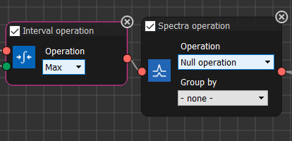
We won't use the next node in our calculations so we could just delete it, alternatively set it to Null Operation.
Press Run again, so that the values propagate along our path so far.
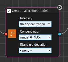
In keeping with plotting concentration as a function of intensity from the previous tutorial, select Na Concentration (or whatever you called the column when you added it to the meta data above) in the Intensity dropdown, and range_0_MAX in the Concentration dropdown.
Finally, press Run again.
A scatter plot similar to below should appear underneath the black recipe area. The information is there, but the defaults for the chart are not all that helpful!
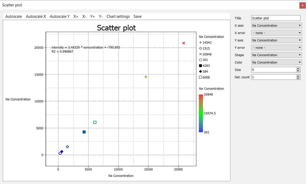
Adjusting the X Axis, Y Axis, Shape and Colo(u)r will give something more useful/familiar.
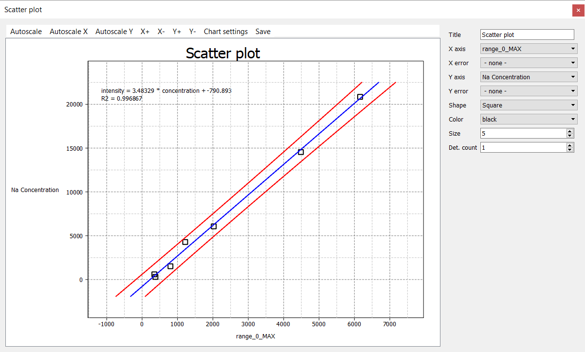
This curve varies slightly from the one we derived in the previous tutorial as this one isn't forcing the curve through 0
Where to from here?
The AtomAnalyzer software has a large number of nodes which we haven't explored here, allowing some powerful techniques to be applied to LIBS spectra. Feel free to explore these.
In the next tutorial, we will utilise another tool for LIBS analysis - Python.