LIBS Info: Tutorial 2: LIBS Analysis with a Spreadsheet
Introduction
$\begin{aligned} I = X Y \frac{g_k A_{ki} C}{U(T)} K(a,x) e^{\frac{-E_k}{kT}} \end{aligned} $
In this Tutorial, we will utilise the LIBS Equation from the previous Tutorial, to begin to analyse some samples.
For this work, we will use some spectra obtain from OREAS Geological Samples. To facilitate the analysis the samples were:-
pressed into pellets - to reduce the variability in plasma temperature by ensure that the level of dust was kept at a minimum (pressed) and the sample surface was kept uniform (pellets)
subjected to multiple laser pulses across the sample surface - to obtain an average spectra for analysis
The final spreadsheet file can be downloaded from this link
Importing the data
For this work we will use the following samples, and analyse for Sodium (Na)
| Sample | Na. Conc (ppm) |
|---|---|
| OREAS45e | 594 |
| OREAS501b | 20848 |
| OREAS601 | 14543 |
| OREAS921 | 6068 |
| OREAS603 | 4283 |
| OREAS933 | 1515 |
| OREAS903 | 301 |
The spectra were exported from the LIBS software as CSV files and opened in Excel.
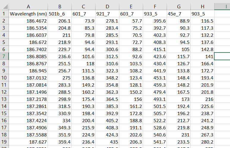
Next we do a simple scatter line plot to get an overall view of our spectra
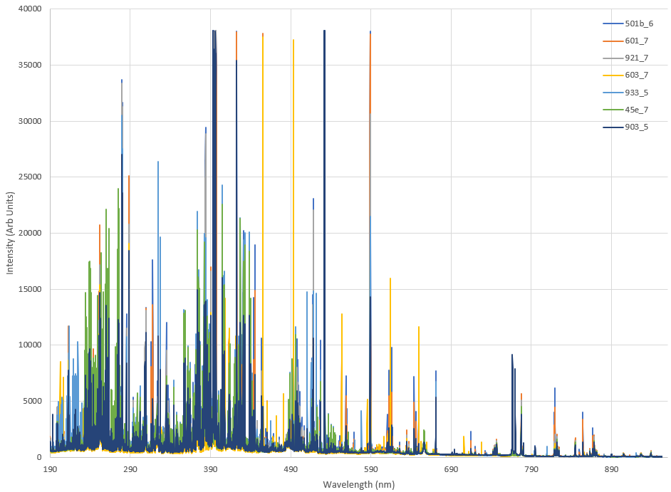
This is a moderately complex LIBS spectra. Some early things to notice
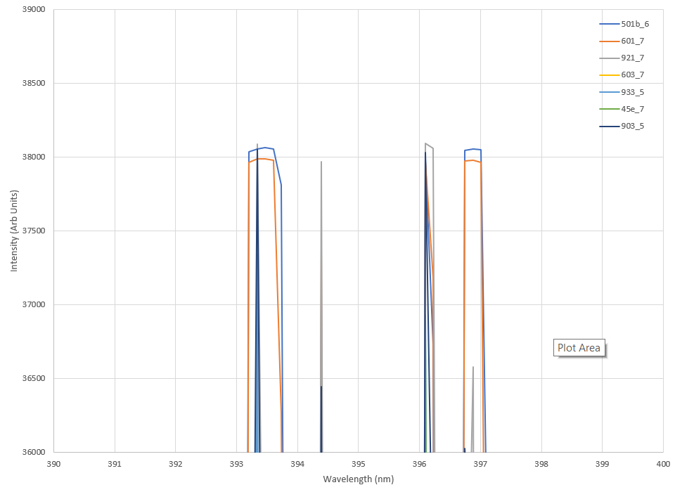
Some of the peaks between 390-590nm end abruptly at about 38000 counts. These are likely to have been too intense for the detection system. They won't have caused any damage, but they won't be any use for analysis purposes.
There are numerous peaks that are not identical across the samples - so there is a reasonable chance we will be able to measure the differences between the spectra, which makes quantitative measurements possible
As discussed in the first Tutorial, this spectra is the combination of the unique spectra of all the elements in the sample. With time, a LIBS user knows the peaks that are unique for elements of interest and is able to examine a spectra such as the above and state that there is Hydrogen, Potassium, Sodium, Calcium, Aluminium, ... present.
Analysing for Sodium
Finding the Sodium Peaks
For most people doing this tutorial, they are not yet at the stage where they can reel off the wavelengths for the 3 or 4 strongest/favourite peaks for an element.
Instead we will use a reference website. As discussed last Tutorial, NIST and AtomTrace both provide LIBS Spectra resources, but we will use the resources at libs-info.com as they provide a list in intensity order.
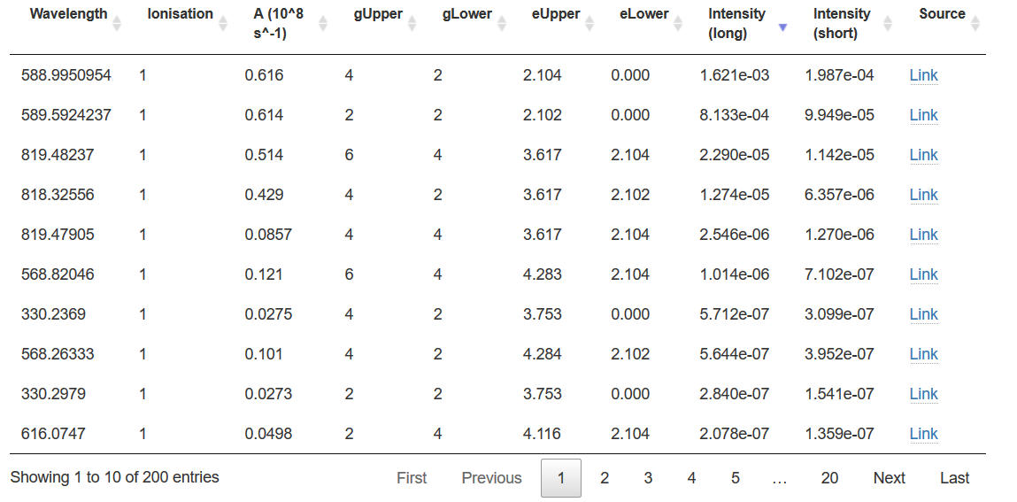
The peaks at 588.995nm, 589.592nm, 819.48nm and 818.33nm look worth investigating. There may also be signal at 568.82nm and 330.24nm, but these are probably ~1000 times weaker, and in parts of the spectrum with peaks from other elements.
589nm and 589.59nm Peaks (Intensity)
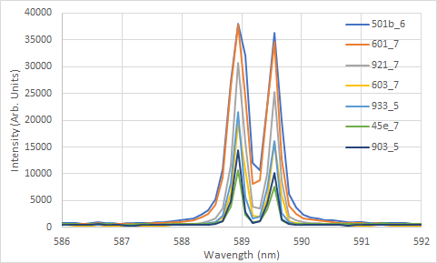 Narrowing down the focus to just the peaks at 589/589.5nm shows that peaks are well separated/resolved from other peaks, but the 589nm peak (and possibly the 589.5nm) are close to that 35000+ Intensity that indicates detector saturation.
| Wavelength (nm) | 501b | 601 | 921 | 603 | 933 | 45e | 903_5 |
|---|---|---|---|---|---|---|---|
| 586.9689 | 731.8 | 648.9 | 494.8 | 357.6 | 476.9 | 563.9 | 405.8 |
| 587.0917 | 747.7 | 667 | 491.6 | 363.7 | 492.5 | 559.6 | 395 |
| 587.2146 | 791.4 | 684.6 | 494.2 | 362.1 | 493.8 | 584.8 | 390 |
| 587.3375 | 812.3 | 703.7 | 513.5 | 372.3 | 472.2 | 582.6 | 413 |
| 587.4603 | 868.6 | 743.3 | 519.7 | 365.2 | 482.5 | 578.7 | 403.4 |
| 587.5831 | 930.6 | 784.2 | 544.9 | 382.6 | 481 | 568.5 | 411.8 |
| 587.7059 | 1001.6 | 830.2 | 559.7 | 387.3 | 509.7 | 591.3 | 410.3 |
| 587.8287 | 1117.9 | 925.5 | 568 | 408.2 | 493.1 | 594.1 | 420 |
| 587.9515 | 1253.1 | 1006.8 | 630.9 | 440.1 | 539.2 | 596.4 | 445.9 |
| 588.0742 | 1427 | 1163.7 | 643.5 | 447.8 | 535.2 | 610.5 | 425.5 |
| 588.197 | 1753.9 | 1393.7 | 725.5 | 483.1 | 582.8 | 606.4 | 450.4 |
| 588.3197 | 2285.8 | 1795.5 | 882.3 | 552.9 | 682.5 | 644.1 | 490.3 |
| 588.4424 | 3246.7 | 2554.9 | 1123.8 | 661.7 | 751.6 | 651.4 | 522.3 |
| 588.5651 | 5196.8 | 4150.5 | 1702.1 | 927.2 | 1019.6 | 743.3 | 646.7 |
| 588.6877 | 10779.7 | 9293.7 | 3552.4 | 1833.5 | 2197.9 | 1196.9 | 1236.1 |
| 588.8104 | 27090 | 26295.4 | 11703.8 | 6185.8 | 8317.5 | 3883.4 | 4873.4 |
| 588.933 | 38021.8 | 37788.1 | 30650.2 | 19405.8 | 21514.3 | 10650.6 | 14327.8 |
| 589.0557 | 32012.9 | 24295.9 | 15719.5 | 10647.9 | 5616 | 2399.1 | 2920.8 |
| 589.1783 | 12066.3 | 8170.9 | 3826.1 | 2203.2 | 1593.9 | 918.5 | 849.4 |
| 589.3009 | 10610.8 | 8723.2 | 3577.7 | 1954.8 | 2072.7 | 1128 | 1194.1 |
| 589.4235 | 22700.8 | 22375.6 | 10041.7 | 5299 | 7315.3 | 3441 | 4307 |
| 589.546 | 36270.7 | 34549.4 | 25271.4 | 15950.2 | 16094.8 | 7597.5 | 10203.2 |
| 589.6686 | 19859.4 | 12638.9 | 8563 | 5865.4 | 2774.8 | 1314.4 | 1453.8 |
| 589.7911 | 6243.6 | 4054.2 | 2051.6 | 1213 | 920.4 | 730.7 | 617.2 |
| 589.9136 | 3633.4 | 2474.4 | 1336.4 | 822.7 | 735.4 | 697 | 568.7 |
| 590.0361 | 2431.9 | 1737.8 | 971.1 | 612.7 | 637.4 | 628 | 467 |
| 590.1586 | 1910.4 | 1427 | 846.7 | 538.6 | 597.3 | 646.7 | 448.6 |
| 590.281 | 1659.5 | 1257 | 742.2 | 512.2 | 600.4 | 634.1 | 450.5 |
| 590.4034 | 1413.7 | 1097 | 711.7 | 477.9 | 571.6 | 643.2 | 441.2 |
| 590.5259 | 1266.9 | 986.1 | 679 | 468.3 | 584.1 | 647.9 | 438.5 |
| 590.6483 | 1134.1 | 893.5 | 609.3 | 468.2 | 541.7 | 607.4 | 422.2 |
| 590.7707 | 1011.4 | 853.4 | 591 | 472.3 | 528.3 | 616.5 | 400.8 |
| 590.8931 | 974.3 | 810 | 561.2 | 400.4 | 533.4 | 624.5 | 423.1 |
| 591.0154 | 916.8 | 778.9 | 551.8 | 376.2 | 547.2 | 628.1 | 430.9 |
| 591.1378 | 865.2 | 735.5 | 549.5 | 396.2 | 557.2 | 646.5 | 417.1 |
| 591.2601 | 880.2 | 746.9 | 567.9 | 408.8 | 617.5 | 737.1 | 456.3 |
| 591.3824 | 872.9 | 725.9 | 609.4 | 417.9 | 648 | 742.2 | 471.2 |
| 591.5047 | 790.4 | 654.1 | 542 | 378.2 | 533.9 | 642.4 | 422.9 |
| 591.627 | 759.4 | 657.9 | 519.8 | 370.3 | 517.5 | 633.9 | 423.3 |
| 591.7492 | 747.3 | 674.2 | 509.9 | 363.1 | 489.5 | 634.9 | 433.2 |
| 591.8715 | 741.6 | 632.8 | 506.1 | 376 | 507.7 | 626.8 | 418.9 |
| 591.9937 | 728.9 | 640.2 | 521.6 | 367.9 | 508.2 | 619.7 | 424.7 |
| 592.1159 | 747.7 | 647.2 | 509.8 | 365.3 | 496.1 | 623.2 | 448.8 |
Choosing the highlighted rows in the table (as these are closest to the peak wavelengths and correspond to the top of the peaks gives us the following)
| Sample | Na Conc (ppm) | 589nm (raw) | 589.5nm (raw) | 587.5nm (raw) | 589nm (net) | 589.5nm (net)} |
|---|---|---|---|---|---|---|
| OREAS45e | 594 | 10650.6 | 7597.5 | 568.5 | 10082.1 | 7029 |
| OREAS501b | 20848 | 38021.8 | 36270.7 | 930.6 | 37091.2 | 35340.1 |
| OREAS601 | 14543 | 37788.1 | 34549.4 | 784.2 | 37003.9 | 33765.2 |
| OREAS921 | 6068 | 30650.2 | 25271.4 | 544.9 | 30105.3 | 24726.5 |
| OREAS603 | 4283 | 19405.8 | 15950.2 | 382.6 | 19023.2 | 15567.6 |
| OREAS933 | 1515 | 21514.3 | 16094.8 | 481 | 21033.3 | 15613.8 |
| OREAS903 | 301 | 14327.8 | 10203.2 | 411.8 | 13916 | 9791.4 |
While it doesn't show in the plot, there is a slightly different baseline for each of different samples. To correct for that, we choose a wavelength without an peaks (here we choose 587.5nm) and subtract this value from the peak heights.
The LIBS Equation, assuming we keep the Temperature constant for all the plasmas can be reduced to
$\begin{aligned} I = X Y \frac{g_k A_{ki} C}{U(T)} K(a,x) e^{\frac{-E_k}{kT}} = b C \end{aligned} $
and traditionally this relationship would be preserved by plotting concentration on the X axis and Intensity on the Y Axis. However, for analysis we are most interested in Concentration, so we will plot concentration on the Y axis and Intensity on the X Axis and look for a fit for
$\begin{aligned} C = \frac{1}{b} I = f I \end{aligned} $
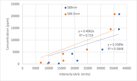
Neither curve is what we might have hoped for. The sharp increase in slope shows that the intensity is not increasing very much for the increase in concentration, suggesting that the detector is saturating.
589nm and 589.59nm Peaks (Peak Area)
Alternatively to Intensity, we can take peak area as our measure. Starting with the LIBS Equation.
$\begin{aligned} \int_{\lambda_{lower}}^{\lambda_{upper}} I d \lambda = \int_{\lambda_{lower}}^{\lambda_{upper}} X Y \frac{g_k A_{ki} C}{U(T)} K(a,x) e^{\frac{-E_k}{kT}} d \lambda = b C \int_{\lambda_{lower}}^{\lambda_{upper}} d \lambda = {constant_0 \quad constant_1 \quad } C \end{aligned} $
or, in words, we can create linear calibration curves plotting the peak area vs concentration
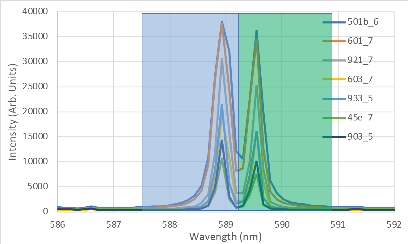
So if we add up the area under the curve (which is equivalent to adding up the individual intensities for this small sample), then that will give the intensity sum under the total curve. As with the peak intensities, we should subtract off the 'pedestal' (the peak area offset) to get a net peak area.
In this case, because there are no detectable peaks for any other elements between the 589nm and 589.5nm peaks, we can also investigate the area of the two peaks combined.
| Sample | Na Conc (ppm) | 589nm Peak Area | 589.5nm Peak Area | Both Peaks together |
|---|---|---|---|---|
| OREAS45e | 594 | 17823.5 | 11790 | 29815.7 |
| OREAS501b | 20848 | 135766.5 | 101219.2 | 223851.3 |
| OREAS601 | 14543 | 118193.4 | 85745 | 192873.4 |
| OREAS921 | 6068 | 68781.8 | 49618.6 | 114770.5 |
| OREAS603 | 4283 | 41565.5 | 30225.4 | 69756.9 |
| OREAS933 | 1515 | 40173 | 27801.2 | 66853.7 |
| OREAS903 | 301 | 23859.6 | 16422.1 | 39287.4 |
Again, plotting concentration on the y axis, peak area this time on the x axis gives
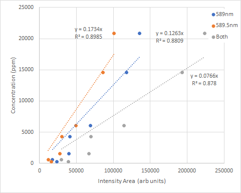
The $R^{2}$ values show a significant improvement, although probably still not as good as we might have hoped.
To note, while the peak intensities showed saturation, this is significantly less present in the peak areas making them often a better candidate for calibration curves.
818.3nm and 819.4nm Na Peaks
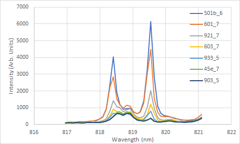 For comparison, let's look at the Na peaks in the 817-821nm region. The Na Peaks at 818.3nm and 819.4nm are quite well resolved, but there is a peak from an unidentified element in the 818.8nm region.
Repeating the analysis using the Peak Intensity gives
| Sample | Na Conc (ppm) | 818.3nm (raw) | 819.4nm (raw) | 817.5nm | 818.3nm (net) | 819.4nm (net) |
|---|---|---|---|---|---|---|
| OREAS45e | 594 | 502.6 | 345.8 | 107.1 | 395.5 | 238.7 |
| OREAS501b | 20848 | 4049.6 | 6160.1 | 142.9 | 3906.7 | 6017.2 |
| OREAS601 | 14543 | 2855.1 | 4487.6 | 164.1 | 2691 | 4323.5 |
| OREAS921 | 6068 | 1417.5 | 2024 | 117.2 | 1300.3 | 1906.8 |
| OREAS603 | 4283 | 920.4 | 1217.5 | 110.5 | 809.9 | 1107 |
| OREAS933 | 1515 | 675.3 | 801 | 95.3 | 580 | 705.7 |
| OREAS903 | 301 | 477.3 | 377.1 | 90.6 | 386.7 | 286.5 |
Which gives the following calibration curves for Peak Intensity
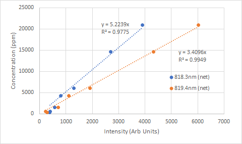
These are considerably more linear than the equivalents around 588nm, with $R^{2}$ or 0.97 or better.
For Comparison, the peak areas are
| Sample | Na Conc (ppm) | 818.3nm | 819.4nm |
|---|---|---|---|
| OREAS45e | 594 | 2628.6 | 991.5 |
| OREAS501b | 20848 | 11246.5 | 15645.2 |
| OREAS601 | 14543 | 9285.6 | 11479.6 |
| OREAS921 | 6068 | 4936 | 4942.7 |
| OREAS603 | 4283 | 3364.6 | 2979.2 |
| OREAS933 | 1515 | 2812.6 | 1923 |
| OREAS903 | 301 | 2477.1 | 1061.5 |
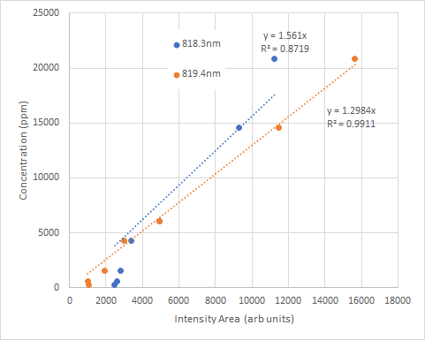
In this case, the Peak Area calibration curve $R^{2}$ are still quite respectable, but not as good as the Peak Intensity curves.
Analysis Performance
While a $R^{2} > 0.95$ is nice to have, in practice what is more important is the analytical performance of our calibration curve.
In these tutorials we will look at a range of methods, two comparatively simple measures are
- detection limit - estimates the smallest concentration that can be detected
- linear regression uncertainty - estimates uncertainty in measurement along the calibration curve
Detection Limit (or Limit of Detection = LOD)
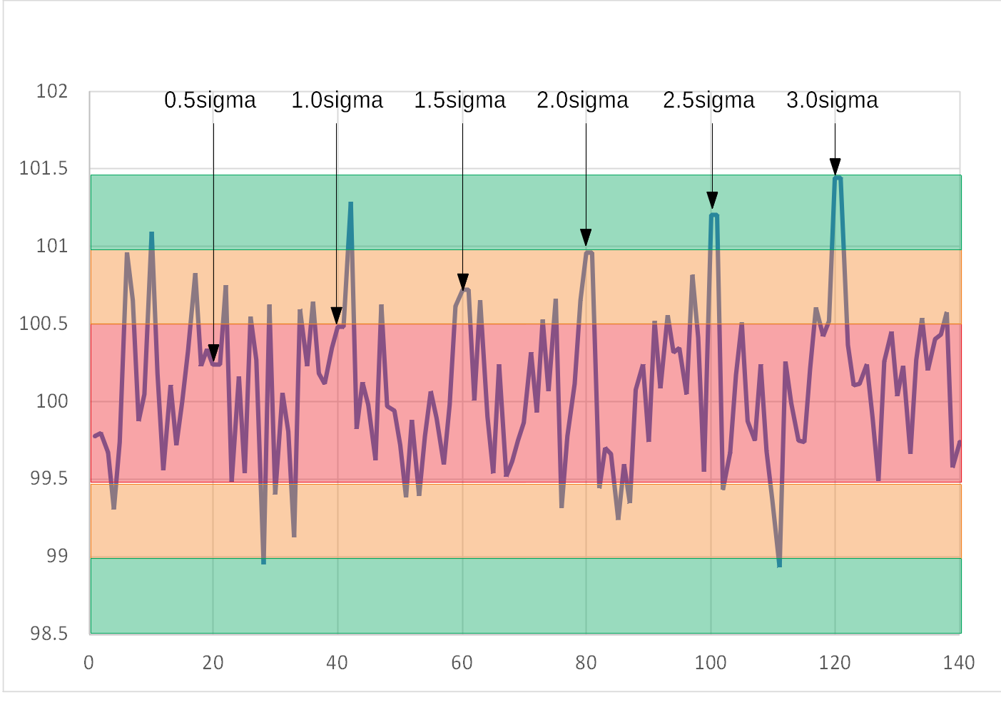
Convention uses the figure of $3 \sigma $, where $\sigma$ is an estimate of the noise in the spectra, as the intensity of the smallest feature that can be detected.
While hardly a proof, the image below shows peaks that are increasing multiples of $\sigma$. The background using noise with a gaussian distribution with a standard deviation of 0.5. The peak at $3 \sigma $ is only just the strongest peak shown
Return to our equation above, where we have included the units for f
$\begin{aligned} C = \frac{1}{b} I = f (units = \frac{Concentration}{Intensity}) I \end{aligned} $
we note that our smallest peak that we are confident is above the noise represents a concentration of
$\begin{aligned} LOD = f (units = \frac{Concentration}{Intensity}) 3 \sigma = 3 \sigma (slope) \end{aligned} $
This makes intuitive sense, the calibration curve with the greatest change in intensity for the smallest change in concentration (that is, with the least slope of a plot of concentration (y axis) vs intensity (x axis) will have the smallest LOD.
Note: the traditional formula of $ \frac{3 \sigma}{slope} $ applies when the calibration curve plots intensity (y axis) vs concentration (x axis)
There are a number of ways to calculate $\sigma$. It is important that the noise is measured near the analysis peak (as the noise can change across the spectrum, particularly if different spectrometers/optica fibres/systems are used to measure different wavelenght regions).
In the calculations here, the standard deviation of the intensity values in the spectrum of the lowest concentration sample (OREAS903) over a range without any obvious peaks - 817-817.8nm for the peaks at 818/819nm and 587-588nm for the peaks at 589nm.
Standard Error (of calibration curve)
Alternatively, the Standard Error of the Regression (S) provides a measure of the typical difference between the predicted concentration (from the calibration curve) and the actual - as measured by the points in the curve. Mathematically, it is defined as
$ S = \sqrt{ \frac{\sum \left( C - f I \right)^2 } {N-1}} $
Evaluating the Performance (Peak Intensity)
For the Peak Intensity calibration curves the performance is
| Peak | Sigma | Slope | $R^2$ | LOD (ppm) | Standard Error (ppm) |
|---|---|---|---|---|---|
| 818.3nm | 7.83 | 5.22 | 0.9775 | 122.6 | 1181.4 |
| 819.4nm | 7.83 | 3.41 | 0.9949 | 80.0 | 562.0 |
| 589nm | 15.93 | 0.34 | 0.5889 | 16.3 | 5054.2 |
| 589.5nm | 15.93 | 0.41 | 0.719 | 19.4 | 4178.2 |
| 589nm (ignore highest conc.) | 15.93 | 0.25 | 0.721 | 11.96 | 3411.1 |
| 589.5nm (ignore highest conc.) | 15.93 | 0.31 | 0.5992 | 14.8 | 2846.2 |
Some things to note
- The Standard Error is not also the calibration curve with the best Limit of Detection
- As noted previously, the calibration curves at 589nm and 589.5nm so some flattening of the curve (likely due to detector saturation), removing the peak of highest concentration improves the performance of the curves (lower LOD and better Standard Error)
Evaluating the Performance (Peak Area)
For the Peak Area calibration curves the performance is
| Peak | Sigma | Slope | $R^2$ | LOD (ppm) | Standard Error (ppm) |
|---|---|---|---|---|---|
| 818.3nm | 7.83 | 1.56 | 0.8719 | 36.6 | 2821.3 |
| 819.4nm | 7.83 | 1.30 | 0.9911 | 30.5 | 743.4 |
| 589nm | 15.93 | 0.126 | 0.8809 | 6.0 | 2720.5 |
| 589.5nm | 15.93 | 0.173 | 0.8985 | 8.3 | 2511.3 |
| 589nm+589.5nm | 15.93 | 0.0766 | 0.878 | 3.7 | 2753.4 |
| 589nm (ignore highest conc.) | 15.93 | 0.104 | 0.8644 | 5.0 | 1983.7 |
| 589.5nm (ignore highest conc.) | 15.93 | 0.145 | 0.8785 | 6.9 | 1877.9 |
| 589nm+589.5nm (ignore highest conc.) | 15.93 | 0.063 | 0.8572 | 3.0 | 2036.2 |
Noting:
- $ \sigma $ is the same, but the peak areas are much larger, leading to better LODs
- However, the average difference between the calibration curve is worse, which is reflected in the Standard Error (and the $ R^2 $)
Best Calibration Curve?
So, after all this work - what is the best calibration curve to use?
In this case, the best depends on the question to be answered.
If the question is, what calibration curve will give the lowest detection limits? Then the answer is using the calibration curve based on the peak area of the combined 589nm and 589.5nm peaks.
If the question is, what calibration curve will give the best overall perfomance? (that is, the expected difference between the calibration and the 'true' value) Then using the calibration curve based on the peak intensity of the 819.4nm peak is the best answer.
What is the best calibration curve will be a question we will keep asking throughout this series.