LIBS Info: Understanding: Element Spectra
Element Spectra
LIBS spectra are immensely complicated involving transient plasma physics, shockwave dynamics, high temperature chemistry and atomic emission. The approach we have taken to produce the indicative spectra for each element do not come close to covering all of these effects. The hope is, however, that sufficient has been taken into account that elements can be identified from their indicative spectra
The reason that the indicative spectra are there at all comes from my experiences when starting out in LIBS - it was extremely difficult to identify many of the elements from their spectra.
Take Aluminium for example: - A little experience shows that one is unlikely to see more than a single ionisation. So, putting Al i-ii into NIST gives
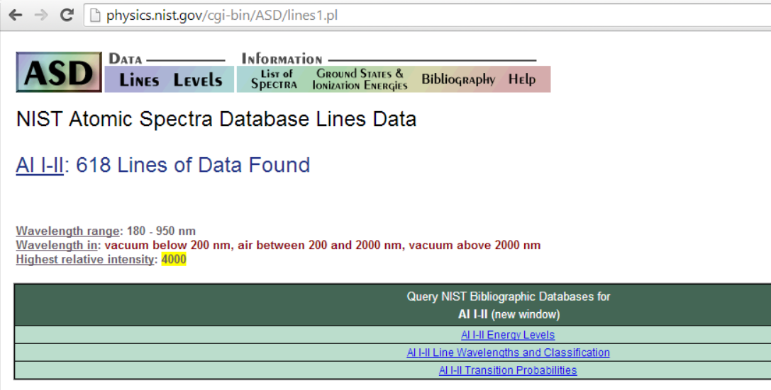
Great, so we should be looking for the peak at 281.6185nm (and the peak at 280.1178nm also looks promising!).
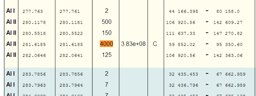
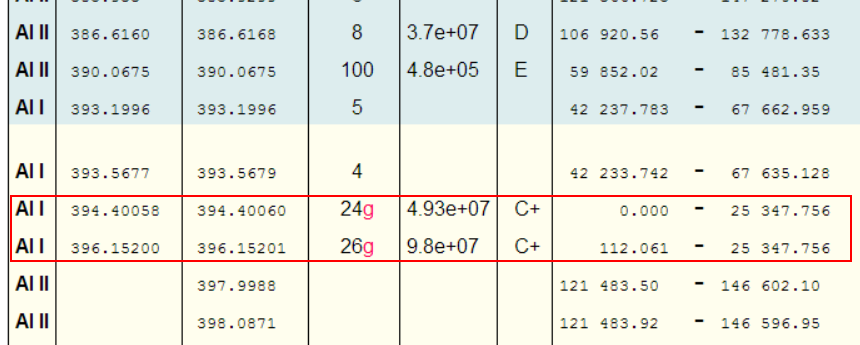
Even limiting things to just Al I, shows the highest relative intensity peaks as
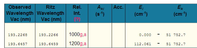
Why would one pay any attention to these peaks? [which are typically the brightest Al peaks in any LIBS spectra!]
The peak intensities come from 2 main equations. The first of these describes the intensity of a peak in a LIBS (or other atomic emission spectrum where self absorption can be neglected) and is given by
$$ \begin{aligned} I=a C \frac{g_{k} A_{ki}}{U(T)} e^{- \frac{E_{k}}{kT}} \end{aligned} $$
where $$ \begin{aligned} I &=Intensity \\ c &=Concentration \\ a &=scaling \quad factor \\ T &=temperature \\ U(T) &= partition\quad function \\ A &= Einstein\quad Coefficient \\ g_{i} &= Upper\quad level \ quad degeneracy \\ E_{ij} &= Upper\quad level \quad energy \\ k &=Boltzmann's \quad constant \\ \end{aligned} $$
However, this only describes the instantaneous intensity. In a LIBS plasma, the temperature is changing - hence the peak intensity is constantly changing. To add to the complexity, what is recorded as the spectrum is the integration of this intensity over the integration time/gate width of the detector. A typical LIBS plasma lasts 100us, but the integration time of the Sony ILX554B CCD (commonly used in Ocean Optics/Avantes based spectrometers) is as long as 1ms.
Also, while the total concentration of an element in the plasma remains constant, the concentration distribution amongst the ions of that element is a function of the temperature and the electron density. This distribution is described by the Saha-Boltzmann equation
$$ \begin{aligned} n_e \frac{n_i}{n_a} = 2 \frac{ \left ( 2 \pi m_e k T \right )^{ \frac{3}{2} }}{h^3} \frac{U_i(T)}{U_a(T)} e^{-\frac{E_{ion}}{kT}} \end{aligned} $$ where $$ \begin{aligned} h &=Plank's \quad Constant \\ n_e &=Electron \quad Density \\ n_i &=number\quad density \quad ions \\ n_a &=number\quad density \quad atoms \\ U_a(T) &= partition\quad function \quad atoms \\ U_i(T) &= partition\quad function \quad ions \\ m_e &= electron\quad mass \\ E_{ion} &= Ionisation \quad Energy \\ \end{aligned} $$
Combine this with conservation of charge
$$ \begin{aligned} n_e = n_i \end{aligned} $$
conservation of matter
$$ \begin{aligned} n_i + n_a = n = constant \end{aligned} $$
we have, for a given Temperature (T) and n, 3 (non-linear) equations in 3 unknowns.
Looking at the different parts of the Intensity equation above for a couple of elements shows some of the complexities involved.
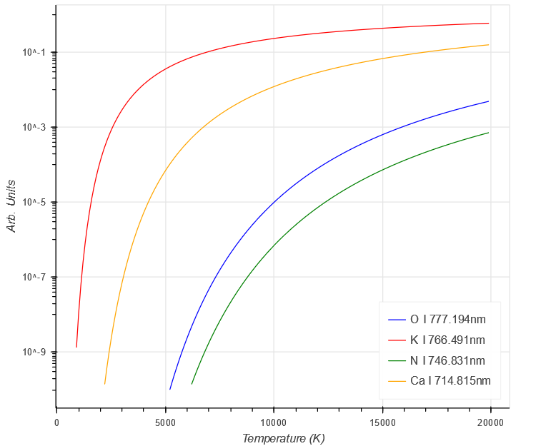
Firstly, the intensity due to the population of the energy levels, which shows a steady increase with temperature. Different elements have different intensities due to the higher values of $ E_{k} $ in O and N, compared to Ca and K.
 $ \begin{aligned}
g_{k} A_{ki} e^{- \frac{E_{k}}{kT}}
\end{aligned} $
$ \begin{aligned}
g_{k} A_{ki} e^{- \frac{E_{k}}{kT}}
\end{aligned} $
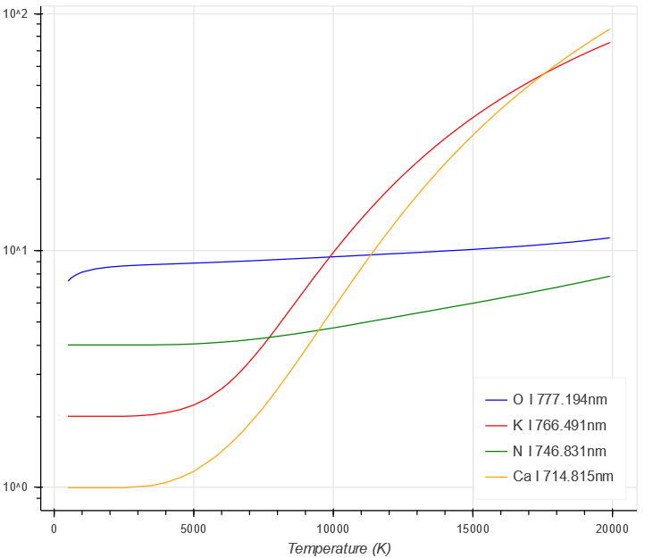
Next, the partition function also shows a steady increase with temperature. [Note this is in the denominator of the peak intensity equation]
 $ \begin{aligned}
U(T)
\end{aligned} $
$ \begin{aligned}
U(T)
\end{aligned} $
With increasing temperature, a greater fraction of the element is ionised, hence the fraction in the neutral decreases.
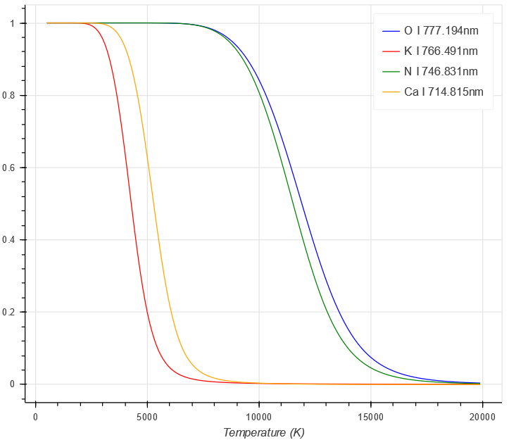 $ \begin{aligned}
Saha-Boltzmann
\end{aligned} $
$ \begin{aligned}
Saha-Boltzmann
\end{aligned} $
The final result shows the complicated behaviour involved
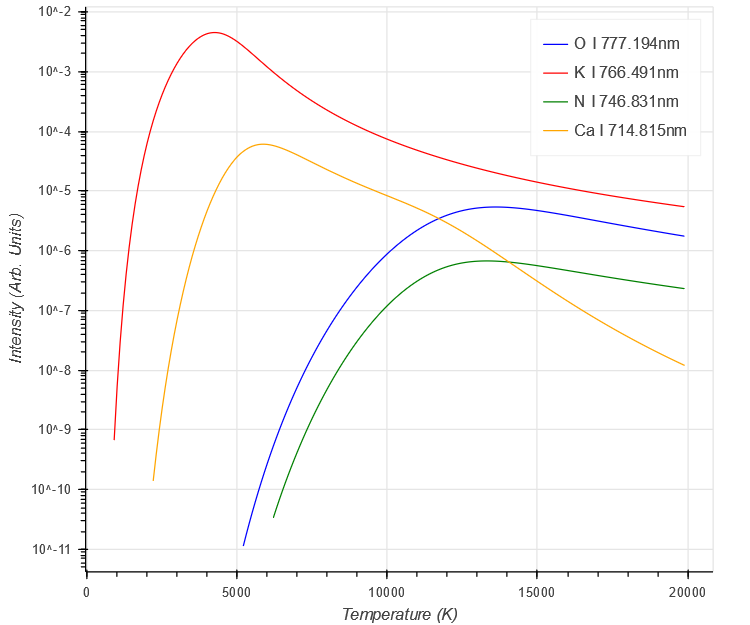 $ \begin{aligned}
I=a C \frac{g_{k} A_{ki}}{U(T)} e^{- \frac{E_{k}}{kT}}
\end{aligned} $
$ \begin{aligned}
I=a C \frac{g_{k} A_{ki}}{U(T)} e^{- \frac{E_{k}}{kT}}
\end{aligned} $
Finally, we model the plasma temperature as a function of time (in microseconds) by
$$ \begin{aligned} T(t) = T_0 + T_1 e^{-a_1 t} + T_2 e^{-a_2 t} \end{aligned} $$
This function DOES NOT have any theoretical basis. However, it did give peak heights/indicative spectra that were closest what had been observed. The closest match came by using $$ \begin{aligned} T_0 &=550K \\ T_1 &=3000K \\ T_2 &=3000K \\ a_1 &= 0.99 \\ a_2 &= 0.001 \\ n &= 1 \text{ } 10^{22} m^{-3}\\ \end{aligned} $$
Putting this together, the intensities in the tables are $$ \begin{aligned} I=\int_0^{t_f} {a C(t) \frac{g_{k} A_{ki}}{U(T(t))} e^{- \frac{E_{k}}{kT(t)}}} \end{aligned} $$
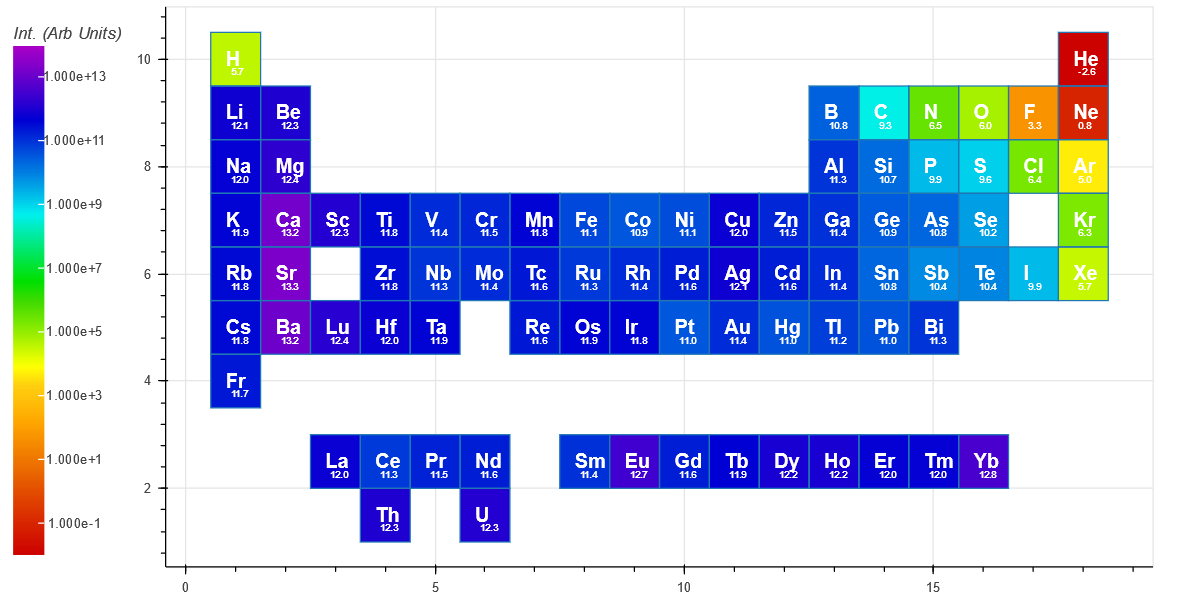
The Intensity(short) is indicative of an intensified CCD or similar and has an integration time ($ t_f $) of 1 microsecond.
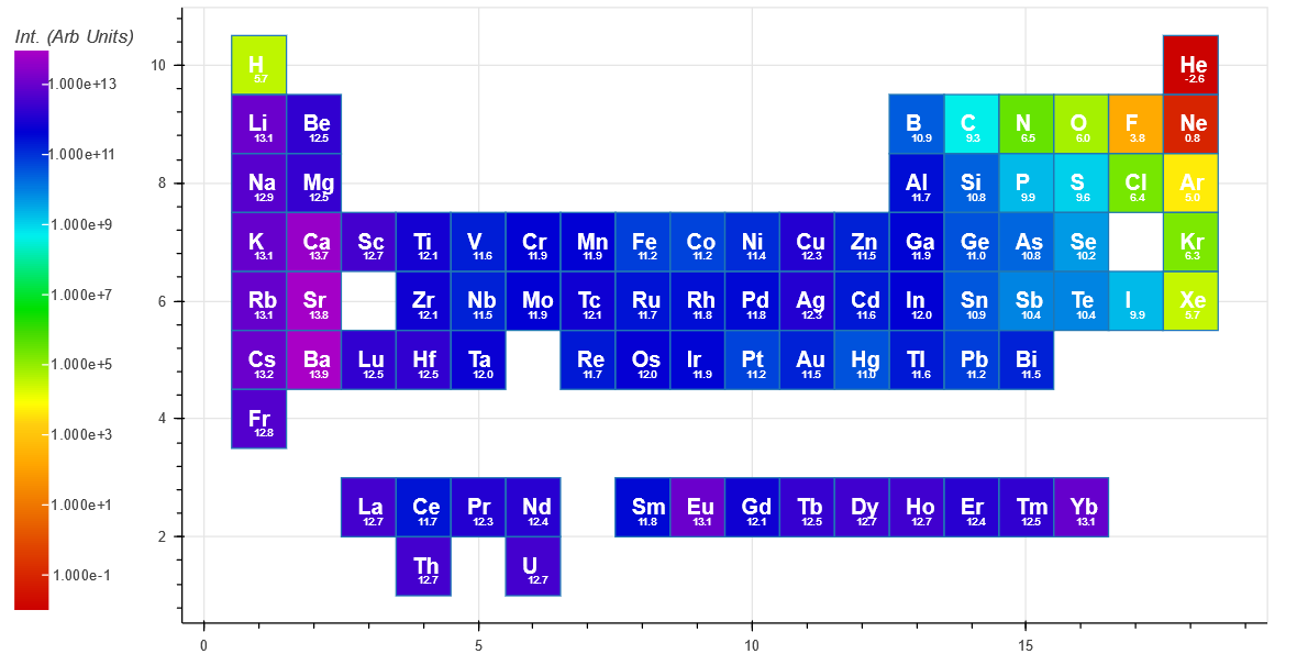
The Intensity(long) has an integration time ($ t_f $) of 100 microsecond, and is more representative of the spectra from an Ocean Optics or Avantes spectrometer based system.
For comparison, the peak with the highest intensity for each element is shown below for short integration (top periodic table) and long integration (bottom periodic table). Both show a trend of decreasing intensity when traveling from left to right on the periodic table. [The small number under each Element symbol is the log10 of the intensity]